Linear waveguide taper by eigenmode expansion

A photonic chip guides light in waveguides, strips of silicon a fraction of a micrometre wide that hold light by total internal reflection. Light travels along a waveguide as modes, field patterns that keep their shape: the fundamental mode, TE0, has one lobe across the strip, and a wide strip also carries TE2, with three. Circuits often pass light from a narrow routing strip to a wide one, at a splitter or a grating coupler, through a taper, a strip whose width changes along its length. An abrupt step hands only part of the power to the wide strip's TE0; the rest goes into TE2 and into radiation that leaves the guide. A taper that widens slowly lets TE0 reshape as it goes, so the power stays in TE0: the taper is then called adiabatic. The figure of merit is the TE0 transmission, the fraction of the input power that leaves in TE0, against the taper's length: short tapers keep 60 to 90 % of it, long ones above 99 %, and a good design is the shortest that meets its target.

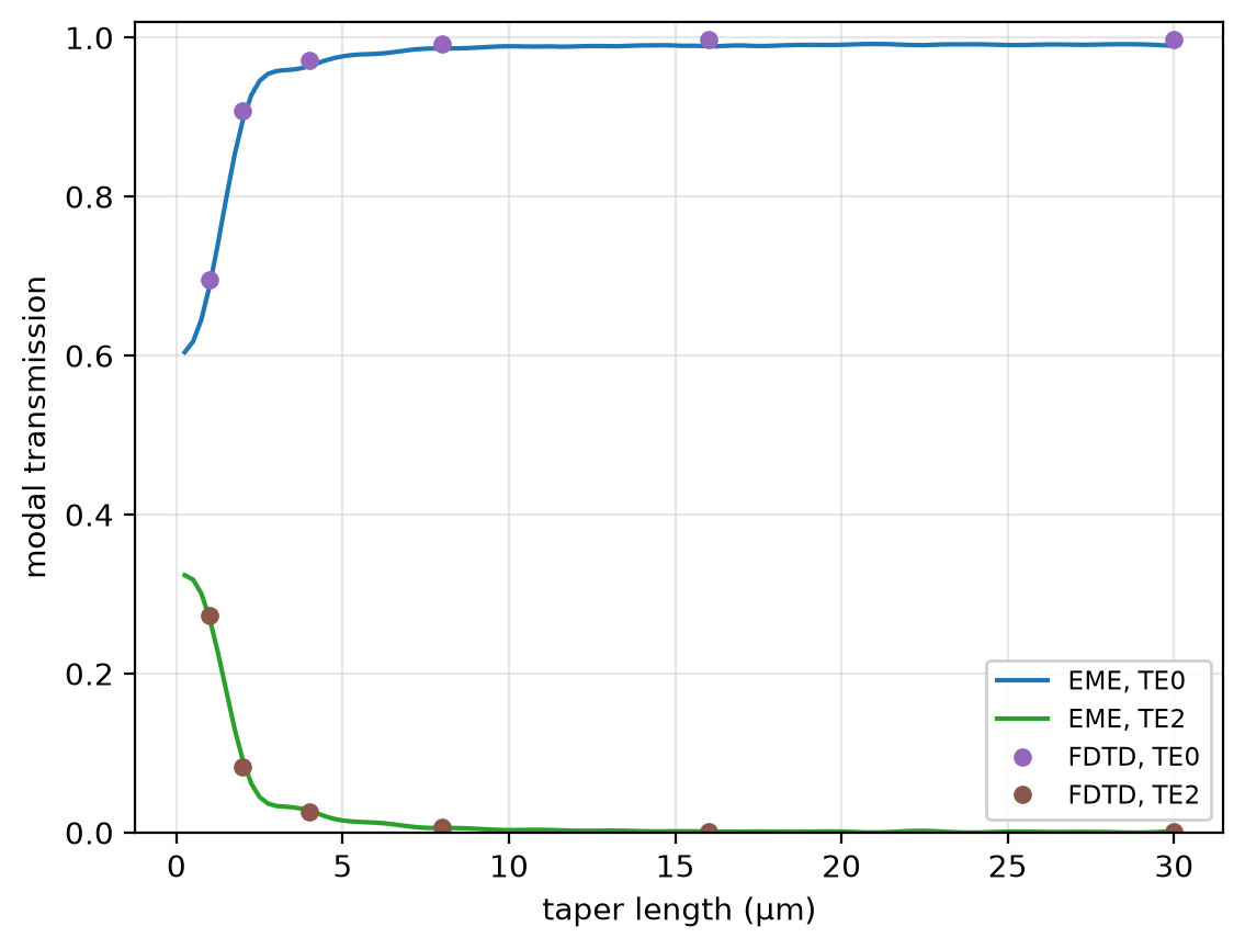
This notebook computes a 0.5 to 2 µm taper's TE0 transmission against length by eigenmode expansion (EME) and checks six lengths with PhotonHub FDTD; there is no paper. At 2 µm the EME reads 0.8967 against 0.9084 from FDTD, on a coarse mesh that sets the input mode's index 1.4 % low; the finest EME reads 0.9004.

Parameters

EME cuts the taper into uniform sections, solves the modes of each cross-section, and joins neighbours by matching their fields. The cross-sections do not change with the taper's length, so they are solved once and each length is a product of small matrices; FDTD steps the whole 3D field again for every length. Each cross-section sits in a box with metal walls, solved on half its width, since a TE0 input keeps the taper's mirror symmetry. It keeps every guided mode and 30 box modes, which carry the short taper's radiation. Forty sections on a 0.04 µm mesh keep the solves to minutes. FDTD uses 15 cells per wavelength, within 0.12 percentage points of 30 cells in TE0 and 0.18 in TE2.

import matplotlib.pyplot as plt
import numpy as np

import photonhub as ph
from photonhub.analysis import VectorModeSolver, cascade, interface_smatrix, propagation_smatrix

# design
w_in = 0.5  # input strip width (µm)
w_out = 2.0  # output strip width (µm)
h = 0.22  # silicon thickness (µm)
n_si = 3.48  # silicon index, constant
n_sio2 = 1.44  # oxide index, on every side, constant
wlen0 = 1.55  # wavelength (µm)

# EME choices
dl_eme = 0.04  # cross-section mesh (µm)
box_w = 5.0  # box width (µm), metal walls
box_h = 3.0  # box height (µm)
n_cells = 40  # uniform sections along the taper
n_box = 30  # box modes per cross-section, besides the guided modes
lengths = np.arange(0.25, 30.01, 0.25)  # taper lengths swept (µm)

# FDTD choices
fdtd_lengths = [1.0, 2.0, 4.0, 8.0, 16.0, 30.0]  # taper lengths run (µm)
L = fdtd_lengths[1]  # the length whose field is shown (µm)
cells_per_wlen = 15  # mesh cells per wavelength, in each medium
lead = 1.5  # straight strip before each port (µm)
clearance = (1.2, 1.0)  # silicon to PML, across and above (µm)
pml = 12  # PML layers
shutoff = 1e-7  # field decay that ends the run
f0 = ph.c0 / (wlen0 * 1e-6)  # frequency (Hz)

Geometry

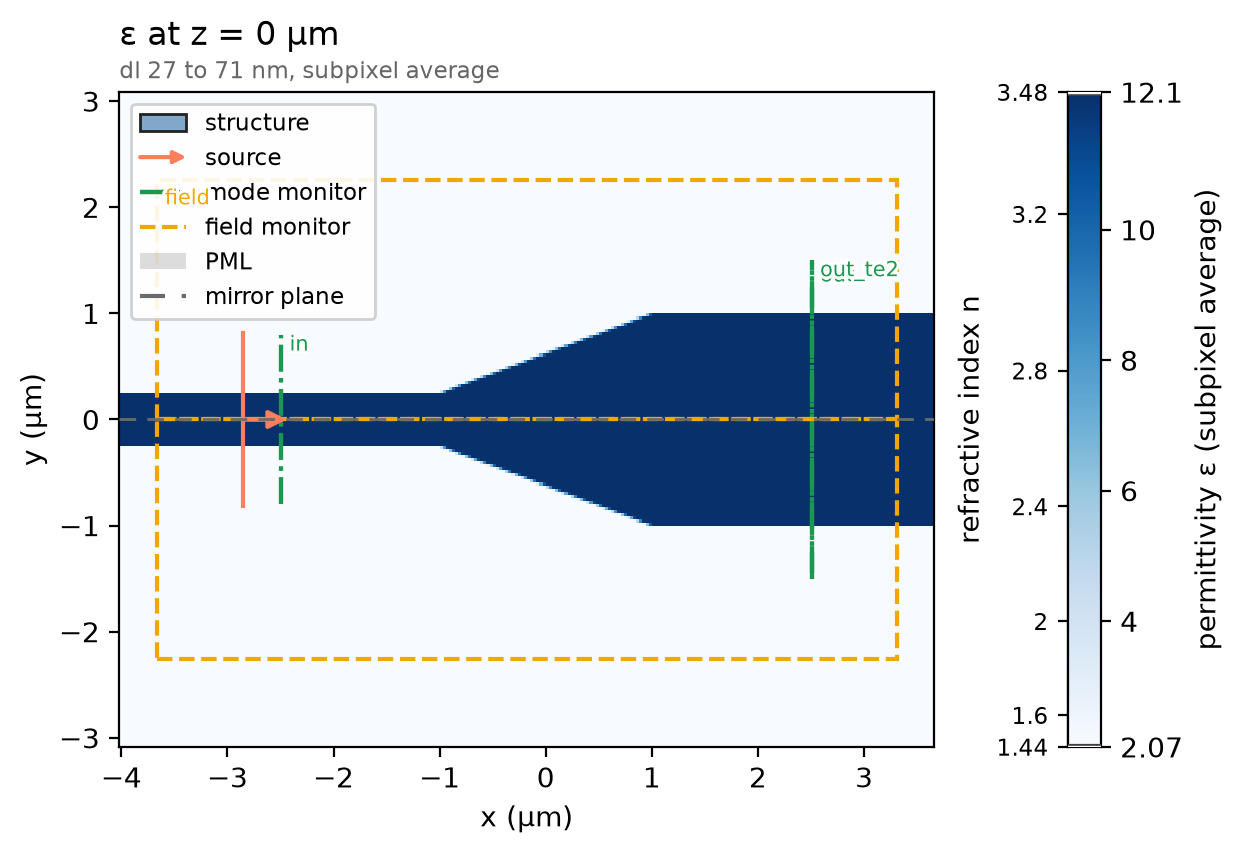
The EME taper is a staircase: the input and output strips as its two ports, and between them 40 uniform sections, each as wide as the taper at its centre.

centres = (np.arange(n_cells) + 0.5) / n_cells  # section centres, 0 to 1 along the taper
widths = [w_in, *(w_in + centres * (w_out - w_in)), w_out]  # core widths (µm)

The FDTD taper is a ph.Polygon, an outline in the chip plane extruded through the silicon, between two straight ph.Box strips; ph.Structure gives each shape its medium. A function draws them at any length.

si = ph.Medium(permittivity=n_si**2)  # silicon, constant index


def taper(L):
    """The FDTD taper of length `L` between its two straight strips."""
    outline = [(-L / 2, -w_in / 2), (L / 2, -w_out / 2), (L / 2, w_out / 2), (-L / 2, w_in / 2)]
    shapes = [
        ph.Polygon(axis="z", vertices_um=outline, slab_bounds_um=(-h / 2, h / 2)),  # the taper
        ph.Box(center_um=(-(L + lead) / 2, 0.0, 0.0), size_um=(lead, w_in, h)),  # input strip
        ph.Box(center_um=((L + lead) / 2, 0.0, 0.0), size_um=(lead, w_out, h)),  # output strip
    ]
    return [ph.Structure(geometry=g, medium=si) for g in shapes]


structures = taper(L)

Simulation

VectorModeSolver.from_rectangular_core samples a centred rectangular core in its box; x_min_symmetry="pec" keeps the half beside the mirror plane, where TE0 and the modes it couples to live. solve finds the guided modes and solve_eme_basis adds the box modes of highest index.

bases = []
for w in widths:
    solver = VectorModeSolver.from_rectangular_core(
        wlen_um=wlen0,
        dl_um=dl_eme,
        core_w_um=w,
        core_h_um=h,
        n_core=n_si,
        n_clad=n_sio2,
        window_w_um=box_w,
        window_h_um=box_h,
        x_min_symmetry="pec",  # half the box: TE0 and the modes it couples to
    )
    n_guided = len(solver.solve(num_modes=8))  # guided modes at this width
    basis = solver.solve_eme_basis(num_guided=n_guided, num_radiation=n_box, pml_cells_xy=(0, 0))
    bases.append(basis)

interface_smatrix matches the fields of two neighbouring bases and returns the junction's scattering matrix. The junctions do not depend on the length, so they are computed once; a length only sets each section's phase, propagation_smatrix, and cascade chains the pieces. By default a junction fits both sides' fields in the least-squares sense. In the unit-power modes of these bases abs(s21[j, 0]) ** 2 is the power from TE0 into output mode j: TE0 is mode 0 and TE2 mode 1.

dl = bases[0][0].dl_x_um  # the cross-section mesh (µm)
junctions = [interface_smatrix(a, b, dl, dl) for a, b in zip(bases, bases[1:])]
T_te0, T_te2 = [], []
for length in lengths:
    segments = [junctions[0]]
    for basis, junction in zip(bases[1:-1], junctions[1:]):
        segments += [propagation_smatrix(basis, length / n_cells), junction]
    s11, s12, s21, s22 = cascade(segments)
    T_te0.append(abs(s21[0, 0]) ** 2)  # TE0 in, TE0 out
    T_te2.append(abs(s21[1, 0]) ** 2)  # TE0 in, TE2 out
print(f"{len(bases)} cross-sections and {len(junctions)} junctions, {len(lengths)} taper lengths")

output

42 cross-sections and 41 junctions, 120 taper lengths

For FDTD, a ph.Port is a plane across a guide: its centre, the axis the light travels along, and the guide's width and thickness. in launches TE0; out reads TE0 and out_te2 TE2, the second mode the mirror plane keeps (mode="TE1"). The SDK sizes the window each mode is read in so the mode is 30 dB down at its edge, with a 20 % margin.

def ports_at(L):
    """The port planes of the taper of length `L`."""
    x_port = L / 2 + lead  # centre to each port plane (µm)
    return [
        ph.Port("in", (-x_port, 0.0, 0.0), "x", w_in, thickness_um=h),
        ph.Port("out", (x_port, 0.0, 0.0), "x", w_out, thickness_um=h),
        ph.Port("out_te2", (x_port, 0.0, 0.0), "x", w_out, thickness_um=h, mode="TE1"),
    ]


ports = ports_at(L)

ph.Simulation holds the setup: ph.Domain fits the box around the taper and continues each strip through the PML, ph.Mesh grades the mesh by cells_per_wlen, two mirror planes keep a quarter of the box, and the run ends when the field has decayed to shutoff.

field = ph.ProfileMonitor.plane("field", "z", 0.0, wlens_um=wlen0)  # the silicon's mid-plane
sim = ph.Simulation(
    domain=ph.Domain(clearance_um=(None, *clearance)),
    mesh=ph.Mesh(cells_per_wlen=cells_per_wlen),
    background=ph.Medium(permittivity=n_sio2**2),  # oxide, constant index
    pml_num_layers=pml,
    structures=structures,
    symmetry=(0, -1, 1),  # mirror planes through the axis and the silicon's middle
    wlens_um=wlen0,
    ports=ports,
    source="in",  # the port that launches TE0
    run=ph.RunSpec(shutoff=shutoff, dft_shutoff=0.0),
    monitors=[field],
)
sim.plot_index(z=0.0)
plt.show()

ph.run_local runs the solver on this computer; ph.cloud.run_quoted runs it on a cloud GPU.

data = ph.run_local(sim, quiet=True)
# On a cloud GPU instead, with GPU and SOLVER from your closed-test guide:
# data = ph.cloud.run_quoted(sim, device=GPU, solver=SOLVER)

Field

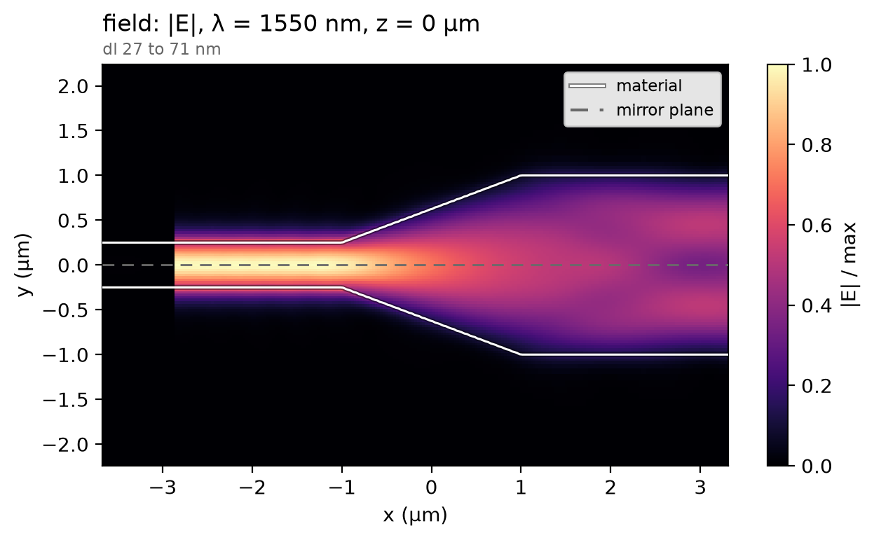
TE0 widens through the taper; the stripes in the wide strip are TE0 and TE2 beating, two modes that travel at different speeds.

data.plot_field("field", field="E", z=0.0)
plt.show()

Result

sim.with_changes swaps in each length's taper and ports, without the field plane; the run above serves for its length.

fdtd_te0, fdtd_te2 = [], []  # FDTD modal transmission at each length
for length in fdtd_lengths:
    sim_length = sim.with_changes(structures=taper(length), ports=ports_at(length), monitors=[])
    out = data if length == L else ph.run_local(sim_length, quiet=True)  # L ran above
    fdtd_te0.append(float(out.transmission("out").sel(f=f0, method="nearest")))
    fdtd_te2.append(float(out.transmission("out_te2").sel(f=f0, method="nearest")))

EME as curves, FDTD as markers; the print lists both TE0 values.

ph.viz.plot_comparison(
    lengths,
    {
        "EME, TE0": T_te0,
        "EME, TE2": T_te2,
        "FDTD, TE0": (fdtd_lengths, fdtd_te0),
        "FDTD, TE2": (fdtd_lengths, fdtd_te2),
    },
    points=("FDTD, TE0", "FDTD, TE2"),  # discrete runs: markers, no joining line
    xlabel="taper length (µm)",
    ylabel="modal transmission",
    ylim=(0.0, 1.02),
)
plt.show()
eme_te0 = [T_te0[int(np.argmin(abs(lengths - x)))] for x in fdtd_lengths]  # EME at those lengths
rows = [f"{x:4g} µm: EME {e:.4f}, FDTD {t:.4f}" for x, e, t in zip(fdtd_lengths, eme_te0, fdtd_te0)]
print(f"TE0 transmission at {wlen0 * 1e3:g} nm\n" + "\n".join(rows))

output

TE0 transmission at 1550 nm
   1 µm: EME 0.6879, FDTD 0.6955
   2 µm: EME 0.8967, FDTD 0.9084
   4 µm: EME 0.9641, FDTD 0.9710
   8 µm: EME 0.9862, FDTD 0.9924
  16 µm: EME 0.9891, FDTD 0.9972
  30 µm: EME 0.9895, FDTD 0.9981

At 40 sections and 30 box modes on a 0.04 µm mesh the EME TE0 transmission of the 2 µm taper reads 0.8967 at 1550 nm; at 160 sections on a 0.015 µm mesh, 0.9004, not shown converged; PhotonHub FDTD at 15 cells per wavelength, 0.9084. EME: metal-walled half boxes, subpixel averaging, default junction; FDTD: graded mesh, contour subpixel averaging, 12 PML layers, two mirror planes; constant indices throughout.