Mode and polarization multiplexer couplers
A single waveguide, a strip of silicon in glass that guides light, can carry several signals at once if each travels in its own mode, a field pattern that keeps its shape along the guide. Modes are named by polarization, TE with the electric field mostly in the chip plane or TM with it mostly vertical, and by order, the number of times the field changes sign across the guide: TE0, TE1, TE2. A mode multiplexer loads each signal into its own mode of one shared bus guide, and a demultiplexer takes each back out. Each coupler must pick one mode and leave the others in the bus. An asymmetric directional coupler does this: a narrow access guide runs beside the wide bus, and light crosses between the guides only when the access guide's fundamental mode travels at the same speed as one bus mode (phase matching). The figures of merit are a channel's excess loss, the power it loses in decibels (dB; 0.1 dB is 2 %), good below 1 dB, and crosstalk, the power reaching a wrong channel, good below -15 to -20 dB.
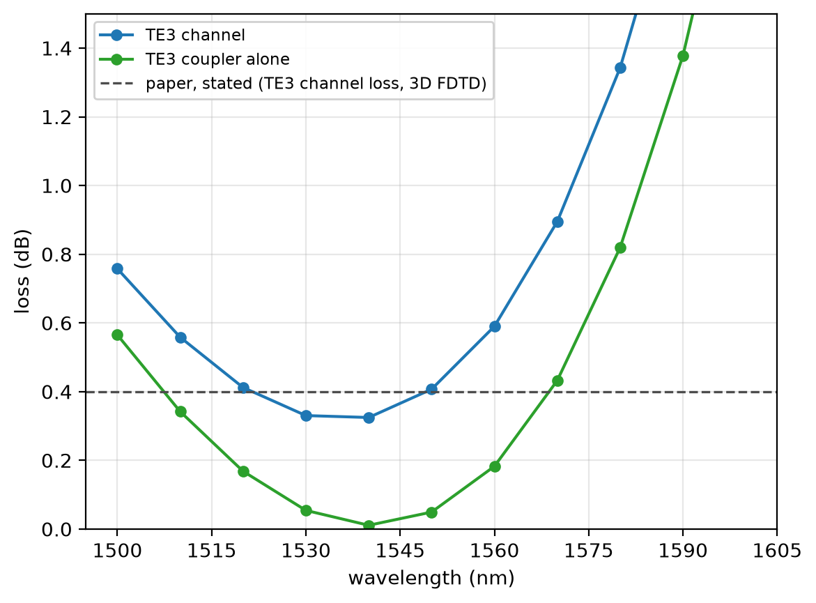
This notebook builds the six couplers of Table 1 of Wang, He and Dai, Laser Photonics Rev. 8, L18 (2014) and follows the TE3 channel of the demultiplexer through the TM2 coupler it passes and its own: 0.407 dB of loss at 1550 nm (0.344 dB at 32 cells per wavelength) against the paper's about 0.4 dB.
Parameters
The design is the paper's Table 1. The paper states neither the indices nor the bends, so both are assumed: constant indices that phase-match all five of its TE width pairs, and raised-cosine bends measured on its Fig. 2. The band is the paper's simulated range. The graded mesh puts a line on every straight guide edge. Oxide above and below makes each coupler mirror symmetric through the silicon's middle, which halves the run.
# design, the paper's Table 1: access width, bus width, gap, coupling length (µm)
table1 = {
    "TM1": (0.400, 1.035, 0.300, 4.7),
    "TM2": (0.400, 1.695, 0.300, 6.7),
    "TM3": (0.400, 2.363, 0.300, 9.0),
    "TE1": (0.400, 0.835, 0.200, 15.5),
    "TE2": (0.406, 1.290, 0.200, 21.3),
    "TE3": (0.379, 1.631, 0.200, 17.6),
}
h = 0.22  # silicon thickness (µm)
n_si = 3.48  # assumed: silicon index, constant
n_sio2 = 1.444  # assumed: oxide index, constant
bend_len = 10.0  # assumed: access bend length, Fig. 2 (µm)
bend_dy = 1.6  # assumed: access bend offset, Fig. 2 (µm)
paper_loss_db = 0.4  # paper, stated TE3 channel loss (dB)
paper_leak_db = -11.0  # paper, stated TE3 into the TM2 port (dB)
# simulation choices
wlen_min = 1.50  # band start (µm)
wlen_max = 1.60  # band end (µm)
n_wlen = 11  # wavelengths read out
cells_per_wlen = 16  # cells per wavelength, in each material
lead = 2.0  # straight guide from each bend to its port (µm)
clearance = 1.2  # silicon to PML, beside and above (µm)
pml = 12  # PML layers
shutoff = 1e-5  # field decay that ends the run

wlen = np.linspace(wlen_min, wlen_max, n_wlen)  # wavelengths (µm)
wlen0 = 0.5 * (wlen_min + wlen_max)  # band centre (µm)
f0 = ph.c0 / (wlen0 * 1e-6)  # band-centre frequency (Hz)
Geometry
A ph.Box is a block given by its centre and size; a ph.Polygon is an
outline in the chip plane (vertices_um, counter-clockwise) extruded through
the silicon (slab_bounds_um); ph.Structure gives each shape its medium.
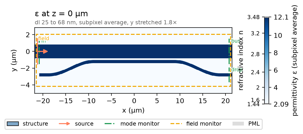
The bus runs along y = 0, the access guide one gap below it, then at each end
a raised-cosine bend and a lead to the port. The runs draw different rows of
Table 1, so the coupler is a function of its row.
def coupler(name):
    wa, wb, gap, Lc = table1[name]
    y_c = -(wb / 2 + gap + wa / 2)  # access guide's axis beside the bus (µm)
    x_end = Lc / 2 + bend_len  # where each bend ends (µm)
    t = np.linspace(0.0, 1.0, 161)
    x = Lc / 2 + bend_len * t
    y = y_c - bend_dy * (1 - np.cos(np.pi * t)) / 2  # a raised cosine
    a = np.arctan2(np.gradient(y), np.gradient(x))  # direction of travel
    right = list(zip(x + wa / 2 * np.sin(a), y - wa / 2 * np.cos(a)))
    left = list(zip(x - wa / 2 * np.sin(a), y + wa / 2 * np.cos(a)))
    bend = right + left[::-1]  # the right-hand bend
    mirror = [(-u, v) for u, v in reversed(bend)]  # the left-hand bend
    slab = (-h / 2, h / 2)
    shapes = [
        ph.Box(center_um=(0.0, 0.0, 0.0), size_um=(2 * (x_end + lead), wb, h)),  # bus
        ph.Box(center_um=(0.0, y_c, 0.0), size_um=(Lc, wa, h)),  # access, beside the bus
        ph.Polygon(axis="z", vertices_um=bend, slab_bounds_um=slab),
        ph.Polygon(axis="z", vertices_um=mirror, slab_bounds_um=slab),
        ph.Box(center_um=(x_end + lead / 2, y_c - bend_dy, 0.0), size_um=(lead, wa, h)),
        ph.Box(center_um=(-x_end - lead / 2, y_c - bend_dy, 0.0), size_um=(lead, wa, h)),
    ]
    si = ph.Medium(permittivity=n_si**2)  # silicon, constant index
    return [ph.Structure(geometry=g, medium=si) for g in shapes]


structures = coupler("TE3")
Simulation
A ph.Port is a plane across a guide: its centre, the axis the light travels
along, the guide's width and thickness, and the mode it launches or reads.
The bus mode arrives from the left at in, as in a demultiplexer; on the
right, drop reads the access guide's fundamental mode and bus what the
coupler passes on, as modal power over the launched power. The SDK sizes the window each mode is solved and read in so
the mode is 30 dB down at its edge, with a 20 % margin.
def ports(name, mode):
    wa, wb, gap, Lc = table1[name]
    x_port = Lc / 2 + bend_len + lead  # the port planes (µm)
    y_drop = -(wb / 2 + gap + wa / 2) - bend_dy  # the access guide's axis there (µm)
    return [
        ph.Port("in", (-x_port, 0.0, 0.0), "x", wb, thickness_um=h, mode=mode),
        ph.Port("bus", (x_port, 0.0, 0.0), "x", wb, thickness_um=h, mode=mode),
        ph.Port("drop", (x_port, y_drop, 0.0), "x", wa, thickness_um=h, mode=mode[:2] + "0"),
    ]
ph.Simulation holds the setup. ph.Domain fits the box around the coupler
and continues each guide through the PML; ph.Mesh grades the mesh by
cells_per_wlen; the run ends when the field has decayed to shutoff. The
two printed indices are the phase matching the coupler rests on.
field = ph.ProfileMonitor.plane("field", "z", 0.0, wlens_um=wlen0)  # the mid-plane
sim = ph.Simulation(
    domain=ph.Domain(clearance_um=clearance),
    mesh=ph.Mesh(cells_per_wlen=cells_per_wlen),
    background=ph.Medium(permittivity=n_sio2**2),  # oxide, constant index
    pml_num_layers=pml,
    structures=structures,
    symmetry=(0, 0, 1),  # TE modes are even about the mid-plane
    wlens_um=wlen,  # wavelengths read out at the ports
    ports=ports("TE3", "TE3"),
    source="in",  # the port that launches the bus mode
    run=ph.RunSpec(shutoff=shutoff),
    monitors=[field],
)
n_bus = float(sim.port_monitors["bus"].mode.n_eff)
n_drop = float(sim.port_monitors["drop"].mode.n_eff)
print(f"TE3 in the bus: n_eff {n_bus:.4f} | TE0 in the access guide: n_eff {n_drop:.4f}")
sim.plot_index(z=0.0)
plt.show()
ph.run_local runs the solver on this computer; ph.cloud.run_quoted runs it
on a cloud GPU. The outputs on this page come from a GPU run of these exact
simulations.
data = ph.run_local(sim, quiet=True)
# On a cloud GPU instead, with GPU and SOLVER from your closed-test guide:
# data = ph.cloud.run_quoted(sim, device=GPU, solver=SOLVER)
Field
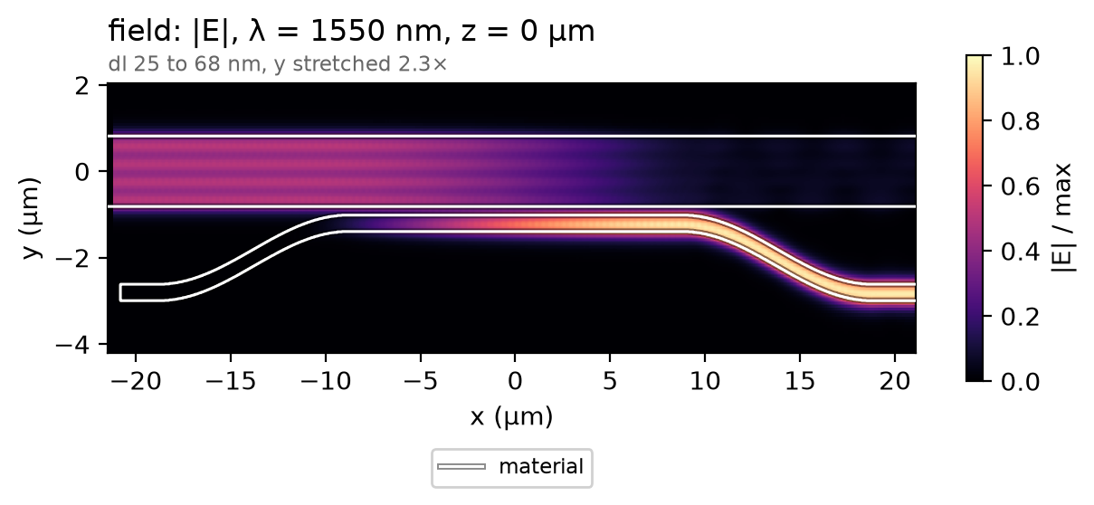
The silicon's mid-plane at 1550 nm. TE3, four lobes across the bus, crosses into the access guide along the coupling section and leaves as TE0.
Result
TE3 passes the TM2 coupler before its own, and that coupler's access TE0,
almost as fast as TE3, takes a share of it: the cause of the paper's -11 dB
crosstalk, per the authors' follow-up,
Opt. Express 22, 12799 (2014).
sim.with_changes rebuilds the simulation around the TM2 coupler; the channel
keeps what it passes times what the TE3 coupler drops. The dashed line is the
paper's stated loss; its licence allows no re-plotting.
sim_x = sim.with_changes(structures=coupler("TM2"), ports=ports("TM2", "TE3"))
data_x = ph.run_local(sim_x, quiet=True)  # TE3 through the TM2 coupler
drop = data.transmission("drop")  # TE3 in the bus to TE0 at the TE3 port
kept = data_x.transmission("bus")  # TE3 left in the bus by the TM2 coupler
leak = data_x.transmission("drop")  # TE3 to TE0 at the TM2 port
ph.viz.plot_comparison(
    drop.wlen_um * 1e3,
    {"TE3 channel": -10 * np.log10(drop * kept), "TE3 coupler alone": -10 * np.log10(drop)},
    stated=(paper_loss_db, "paper, stated (TE3 channel loss, 3D FDTD)"),
    ylabel="loss (dB)",
    ylim=(0.0, 1.5),
)
plt.show()
d, k, x = (float(s.sel(f=f0, method="nearest")) for s in (drop, kept, leak))
loss_db = -10 * np.log10(d * k)  # the channel at 1550 nm (dB)
parts = f"TE3 coupler {-10 * np.log10(d):.3f} dB, TM2 coupler {-10 * np.log10(k):.3f} dB"
leak_db = 10 * np.log10(x)  # TE3 into the TM2 port at 1550 nm (dB)
leak_text = f"TM2 port leak {leak_db:.1f} dB (paper about {paper_leak_db:.0f} dB)"
print(f"TE3 channel at 1550 nm: {loss_db:.3f} dB ({parts}) | {leak_text}")
TE3 channel at 1550 nm: 0.407 dB (TE3 coupler 0.049 dB, TM2 coupler 0.358 dB) | TM2 port leak -11.0 dB (paper about -11 dB)
At 16 cells per wavelength the TE3 channel loss reads 0.407 dB at 1550 nm; at 32 cells, 0.344 dB, not shown converged; the paper's 3D FDTD, about 0.4 dB. From 28 to 32 cells it moves 0.002 dB (0.011 dB across the band), but an earlier step looked as settled. The run uses a graded mesh, contour subpixel averaging, constant indices (no dispersion), 12 PML layers and one mirror plane through the silicon.
Sweep
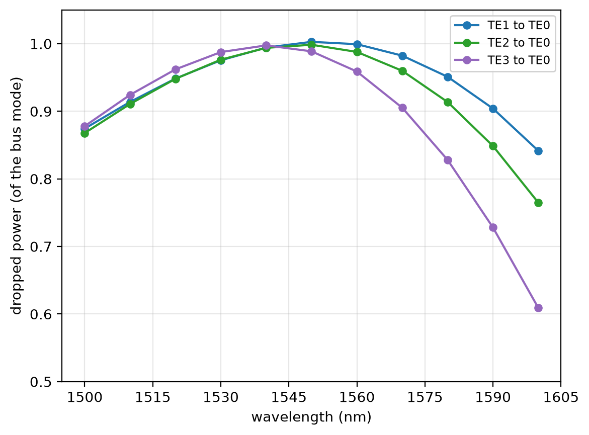
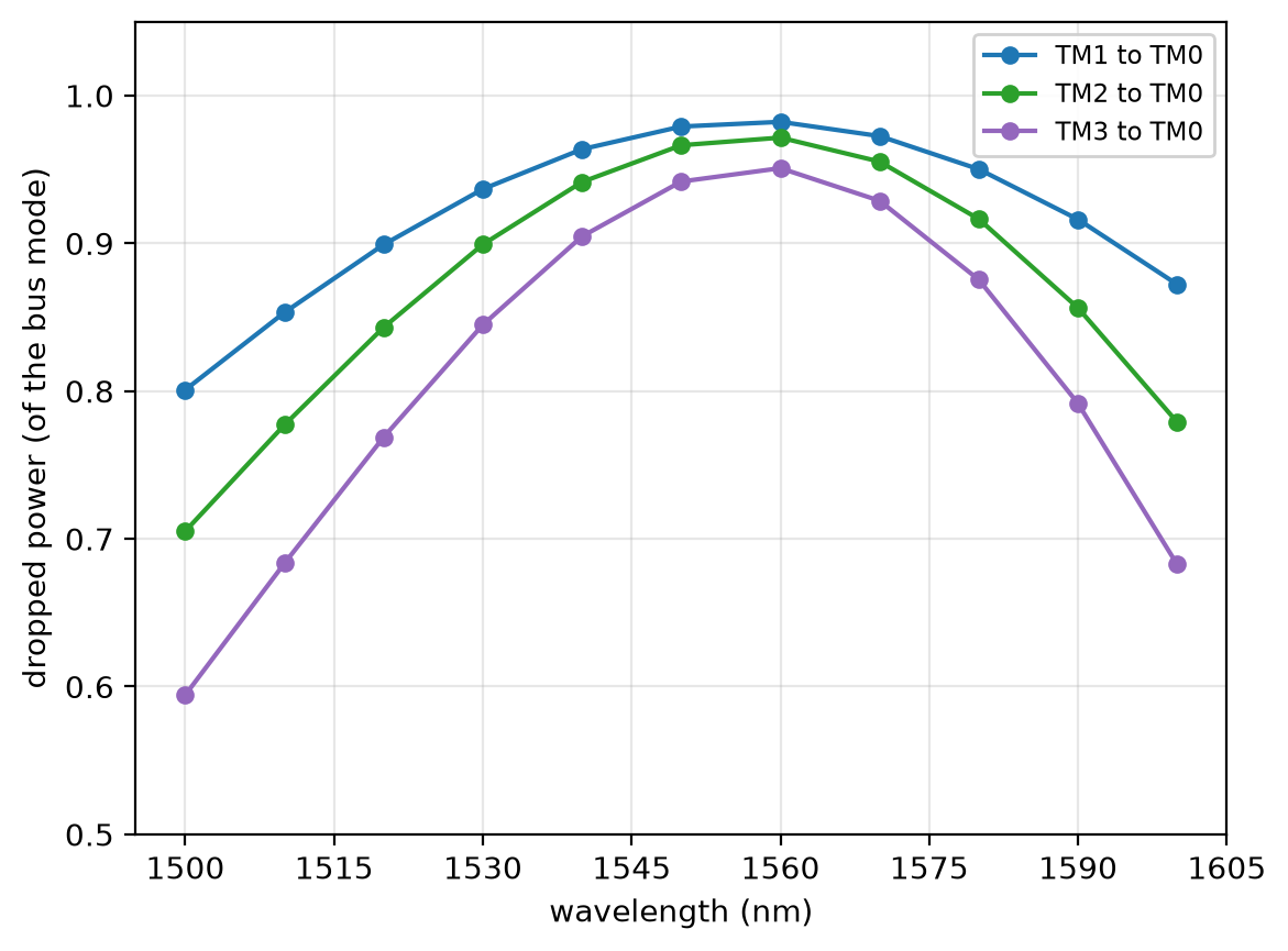
All six couplers with their own mode in the bus, as in the paper's Fig. 2. At 1550 nm the TE couplers drop 0.989 to 1.003 of their mode, above 1 by the readout's floor. The TM couplers peak at 1560 nm, 0.979 to 0.942 at 1550 nm: with constant indices the paper's TM widths sit slightly off phase matching.
drops = {}
for name in table1:
    even = 1 if name.startswith("TE") else -1  # TM modes are odd about the mid-plane
    run = sim.with_changes(structures=coupler(name), ports=ports(name, name), symmetry=(0, 0, even))
    drops[name] = drop if name == "TE3" else ph.run_local(run, quiet=True).transmission("drop")
for pol in ("TE", "TM"):  # one figure per polarization
    ph.viz.plot_comparison(
        drop.wlen_um * 1e3,
        {f"{name} to {pol}0": T for name, T in drops.items() if name.startswith(pol)},
        ylabel="dropped power (of the bus mode)",
        ylim=(0.5, 1.05),
    )
    plt.show()
print(" | ".join(f"{name} {float(T.sel(f=f0, method='nearest')):.3f}" for name, T in drops.items()))